Even though Microsoft Excel has been around for almost 30 years, it’s still the standard.

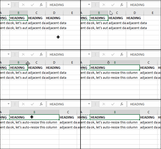
Whether you’re an Excel novice or expert, these 10 tips and tricks will help take your productivity to the next level.

1. Automatically resize a column to the width of the data

This one may be a little obvious to some of you, but it’s surprising how few know about this useful feature in Microsoft Excel. Rather than manually setting the column width, or clicking and dragging the column wider in hopes of revealing all of the content, simply double-click the right border of the column to auto-size it to the width of the widest data contained within!

2. Using AutoFill

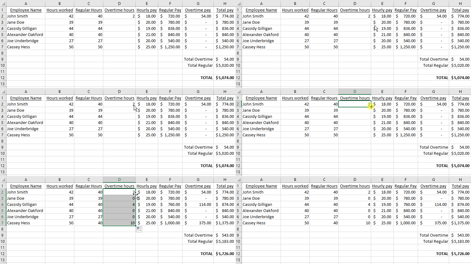
Rather than copying your formula, selecting a range of columns, then pasting — use the fill handle to automate this task. Click on your formula and double-click the small rectangle to the bottom right of the cell to quickly copy it down the column.

This is also useful for working with patterns such as 123, ABC, dates, or even fractions.

For more information and advanced use cases including auto-filling patterns, check out this Microsoft-provided tutorial.

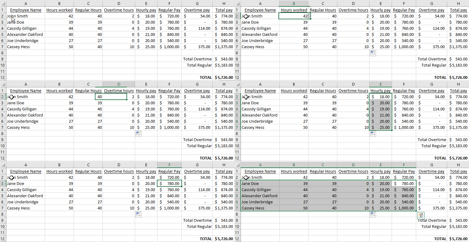
3. Ctrl-Shift to Select

There’s a much faster way to select data than using the mouse and dragging the cursor. Click in the first cell that you want to select and hold down CTRL + Shift followed by a direction key (←↑↓→). Excel will automatically select everything in the direction chosen.

4. Reveal formulas

5. Paste Special to transpose

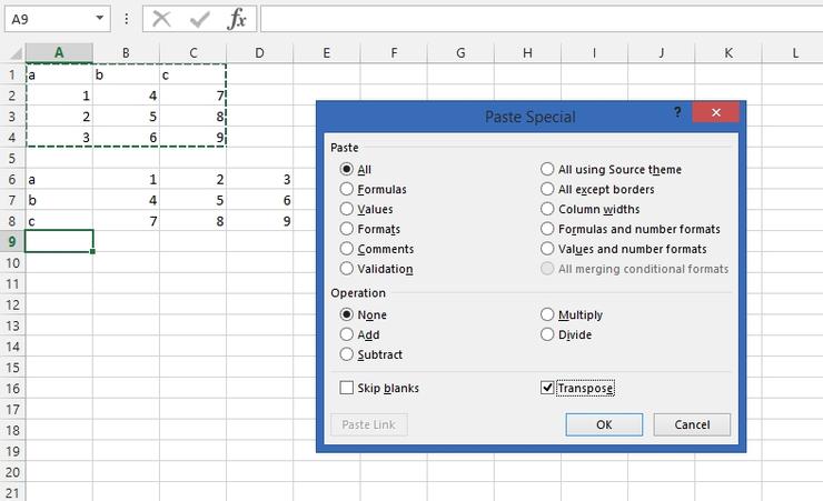
You have a bunch of rows and you want them to be columns or a bunch of columns you want as rows. Sure, you could move them cell-by-cell but why not use the transpose option within the paste special dialogue?

Copy your row or column, right click on your destination and choose Paste Special and check the Transpose box. This will paste your row as a column or column as a row!

6. Paste Special with Formulas

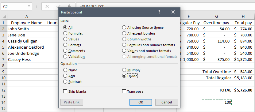
You have a large column of numbers in decimal format and you want to show them as a percentage. Simple, right? The problem is that the number 1 shouldn’t be 100% which is what Excel gives you when you click the Percent style button. You want that 1 to be 1% as it should be which means you’ll be dividing by 100.

That’s where Paste Special comes in. Type 100 into an empty cell and copy it. Then, select all of the numbers that you want divided by 100, right-click and select Paste Special. Check the Divide radio button and voila, your selection has been divided by 100. This also works to instantly add, subtract, and multiply.

For more information, check out this great YouTube tutorial.

7. Use absolute references

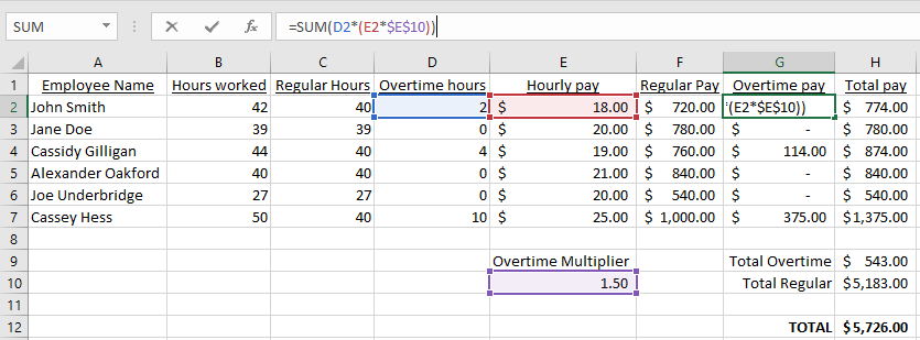
If you have a cell that you need to reference in a formula and don’t want it to automatically increment when using copy-paste or autofill, prefix the column letter and row number with a $. In the above example, we’re using $E$10 to ensure that the overtime multiplier cell E10 never changes in the calculations.

HINT: Have Excel do this for you. Simply select the cell that you want to use in your calculation and press F4. Excel will automatically place $ in the correct spots.

8. Clean up your dataset by removing duplicates

This feature is particularly handy when you’re dealing with larger datasets that come from multiple sources – e.g. contact lists.

To use this function, highlight the row or column you want to remove duplicates from. Then go to Data > Remove Duplicates and you’re all set.

9. Utilize pivot tables to quickly summarize large workbooks

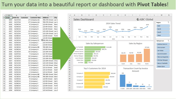
Pivot tables are arguably the most powerful feature in Excel and are a great way to summarize large amounts of data into lists, tables, and charts.
Click the Insert tab followed by Pivot Table to select your data range. If you want assistance selecting the data range, use the recommended pivot table icon instead.

For more information, check out this great YouTube tutorial series.

10. Time saving shortcut keys

Excel, like any great software, has many excellent keyboard shortcuts. Here are some of the best.

F2 : Start editing the current selected cell (much faster than double-clicking).
CTRL + Spacebar : Select the entire column.
Shift + Spacebar : Select the entire row.
F4 : Repeat last action or edit. If you want to repaste something again or repeat a formula.
ALT + = : Automatically SUM() selected cells.
ALT + Enter : Start a new line in the same cell
Ctrl + ; : Inserts today’s date.
Ctrl + Shift + : : Inserts the current time.
Ctrl + Shift + # : Changes the format of a date.
CTRL+ Shift + $ : Applies the currency format to the selected cells.
CTRL + Shift + % : Applies the percentage format to the selected cells.
Ctrl + Ø : Hides the current column.
Ctrl + 9 : Hides the current row.
Ctrl + F6 : Switches between open workbooks (that is, open Excel files in different windows).
Ctrl+` : This combo toggles the view in the sheet to show all the formulas.
Ctrl + PageUp or PageDown : Quick shift between the sheets in the currently open workbook.

10 Essential Microsoft Excel Tips & Tricks